On the Exact Distribution of the Maximum of Absolutely Continuous Dependent Random Variables
Continuous Probability Distributions
A continuous probability distribution is a representation of a variable that can take a continuous range of values.
Learning Objectives
Explain probability density function in continuous probability distribution
Key Takeaways
Key Points
- A probability density function is a function that describes the relative likelihood for a random variable to take on a given value.
- Intuitively, a continuous random variable is the one which can take a continuous range of values — as opposed to a discrete distribution, where the set of possible values for the random variable is at most countable.
- While for a discrete distribution an event with probability zero is impossible (e.g. rolling 3 and a half on a standard die is impossible, and has probability zero), this is not so in the case of a continuous random variable.
Key Terms
- Lebesgue measure: The unique complete translation-invariant measure for the
-algebra which contains all
-cells—in and which assigns a measure to each
-cell equal to that
-cell's volume (as defined in Euclidean geometry: i.e., the volume of the
-cell equals the product of the lengths of its sides).
A continuous probability distribution is a probability distribution that has a probability density function. Mathematicians also call such a distribution "absolutely continuous," since its cumulative distribution function is absolutely continuous with respect to the Lebesgue measure
. If the distribution of
is continuous, then
is called a continuous random variable. There are many examples of continuous probability distributions: normal, uniform, chi-squared, and others.
Intuitively, a continuous random variable is the one which can take a continuous range of values—as opposed to a discrete distribution, in which the set of possible values for the random variable is at most countable. While for a discrete distribution an event with probability zero is impossible (e.g. rolling 3 and a half on a standard die is impossible, and has probability zero), this is not so in the case of a continuous random variable.
For example, if one measures the width of an oak leaf, the result of 3.5 cm is possible; however, it has probability zero because there are uncountably many other potential values even between 3 cm and 4 cm. Each of these individual outcomes has probability zero, yet the probability that the outcome will fall into the interval (3 cm, 4 cm) is nonzero. This apparent paradox is resolved given that the probability that
attains some value within an infinite set, such as an interval, cannot be found by naively adding the probabilities for individual values. Formally, each value has an infinitesimally small probability, which statistically is equivalent to zero.
The definition states that a continuous probability distribution must possess a density; or equivalently, its cumulative distribution function be absolutely continuous. This requirement is stronger than simple continuity of the cumulative distribution function, and there is a special class of distributions—singular distributions, which are neither continuous nor discrete nor a mixture of those. An example is given by the Cantor distribution. Such singular distributions, however, are never encountered in practice.
Probability Density Functions
In theory, a probability density function is a function that describes the relative likelihood for a random variable to take on a given value. The probability for the random variable to fall within a particular region is given by the integral of this variable's density over the region. The probability density function is nonnegative everywhere, and its integral over the entire space is equal to one.
Unlike a probability, a probability density function can take on values greater than one. For example, the uniform distribution on the interval
has probability density
for
and
elsewhere. The standard normal distribution has probability density function:
.

Boxplot Versus Probability Density Function: Boxplot and probability density function of a normal distribution
.
The Uniform Distribution
The continuous uniform distribution is a family of symmetric probability distributions in which all intervals of the same length are equally probable.
Learning Objectives
Contrast sampling from a uniform distribution and from an arbitrary distribution
Key Takeaways
Key Points
- The distribution is often abbreviated
, with
and
being the maximum and minimum values. - The notation for the uniform distribution is:
where
is the lowest value of
and
is the highest value of
. - If
is a value sampled from the standard uniform distribution, then the value
follows the uniform distribution parametrized by
and
. - The uniform distribution is useful for sampling from arbitrary distributions.
Key Terms
- cumulative distribution function: The probability that a real-valued random variable
with a given probability distribution will be found at a value less than or equal to
. - p-value: The probability of obtaining a test statistic at least as extreme as the one that was actually observed, assuming that the null hypothesis is true.
- Box–Muller transformation: A pseudo-random number sampling method for generating pairs of independent, standard, normally distributed (zero expectation, unit variance) random numbers, given a source of uniformly distributed random numbers.
The continuous uniform distribution, or rectangular distribution, is a family of symmetric probability distributions such that for each member of the family all intervals of the same length on the distribution's support are equally probable. The support is defined by the two parameters,
and
, which are its minimum and maximum values. The distribution is often abbreviated
. It is the maximum entropy probability distribution for a random variate
under no constraint other than that it is contained in the distribution's support.
The probability that a uniformly distributed random variable falls within any interval of fixed length is independent of the location of the interval itself (but it is dependent on the interval size), so long as the interval is contained in the distribution's support.
To see this, if
and
is a subinterval of
with fixed
, then, the formula shown:
Is independent of
. This fact motivates the distribution's name.
Applications of the Uniform Distribution
When a
-value is used as a test statistic for a simple null hypothesis, and the distribution of the test statistic is continuous, then the
-value is uniformly distributed between 0 and 1 if the null hypothesis is true. The
-value is the probability of obtaining a test statistic at least as extreme as the one that was actually observed, assuming that the null hypothesis is true. One often "rejects the null hypothesis" when the
-value is less than the predetermined significance level, which is often 0.05 or 0.01, indicating that the observed result would be highly unlikely under the null hypothesis. Many common statistical tests, such as chi-squared tests or Student's
-test, produce test statistics which can be interpreted using
-values.
Sampling from a Uniform Distribution
There are many applications in which it is useful to run simulation experiments. Many programming languages have the ability to generate pseudo-random numbers which are effectively distributed according to the uniform distribution.
If
is a value sampled from the standard uniform distribution, then the value
follows the uniform distribution parametrized by
and
.
Sampling from an Arbitrary Distribution
The uniform distribution is useful for sampling from arbitrary distributions. A general method is the inverse transform sampling method, which uses the cumulative distribution function (CDF) of the target random variable. This method is very useful in theoretical work. Since simulations using this method require inverting the CDF of the target variable, alternative methods have been devised for the cases where the CDF is not known in closed form. One such method is rejection sampling.
The normal distribution is an important example where the inverse transform method is not efficient. However, there is an exact method, the Box–Muller transformation, which uses the inverse transform to convert two independent uniform random variables into two independent normally distributed random variables.
Example
Imagine that the amount of time, in minutes, that a person must wait for a bus is uniformly distributed between 0 and 15 minutes. What is the probability that a person waits fewer than 12.5 minutes?
Let
be the number of minutes a person must wait for a bus.
and
.
. The probability density function is written as:
for
We want to find
.
The probability a person waits less than 12.5 minutes is 0.8333.

Catching a Bus: The Uniform Distribution can be used to calculate probability problems such as the probability of waiting for a bus for a certain amount of time.
The Exponential Distribution
The exponential distribution is a family of continuous probability distributions that describe the time between events in a Poisson process.
Learning Objectives
Apply exponential distribution in describing time for a continuous process
Key Takeaways
Key Points
- The exponential distribution is often concerned with the amount of time until some specific event occurs.
- Exponential variables can also be used to model situations where certain events occur with a constant probability per unit length, such as the distance between mutations on a DNA strand.
- Values for an exponential random variable occur in such a way that there are fewer large values and more small values.
- An important property of the exponential distribution is that it is memoryless.
Key Terms
- Erlang distribution: The distribution of the sum of several independent exponentially distributed variables.
- Poisson process: A stochastic process in which events occur continuously and independently of one another.
The exponential distribution is a family of continuous probability distributions. It describes the time between events in a Poisson process (the process in which events occur continuously and independently at a constant average rate).
The exponential distribution is often concerned with the amount of time until some specific event occurs. For example, the amount of time (beginning now) until an earthquake occurs has an exponential distribution. Other examples include the length (in minutes) of long distance business telephone calls and the amount of time (in months) that a car battery lasts. It could also be shown that the value of the coins in your pocket or purse follows (approximately) an exponential distribution.
Values for an exponential random variable occur in such a way that there are fewer large values and more small values. For example, the amount of money customers spend in one trip to the supermarket follows an exponential distribution. There are more people that spend less money and fewer people that spend large amounts of money.
Properties of the Exponential Distribution
The mean or expected value of an exponentially distributed random variable
, with rate parameter
, is given by the formula:
Example: If you receive phone calls at an average rate of 2 per hour, you can expect to wait approximately thirty minutes for every call.
The variance of
is given by the formula:
In our example, the rate at which you receive phone calls will have a variance of 15 minutes.
Another important property of the exponential distribution is that it is memoryless. This means that if a random variable
is exponentially distributed, its conditional probability obeys the formula:
for all
The conditional probability that we need to wait, for example, more than another 10 seconds before the first arrival, given that the first arrival has not yet happened after 30 seconds, is equal to the initial probability that we need to wait more than 10 seconds for the first arrival. So, if we waited for 30 seconds and the first arrival didn't happen (
), the probability that we'll need to wait another 10 seconds for the first arrival (
) is the same as the initial probability that we need to wait more than 10 seconds for the first arrival (
). The fact that
does not mean that the events
and
are independent.
Applications of the Exponential Distribution
The exponential distribution describes the time for a continuous process to change state. In real-world scenarios, the assumption of a constant rate (or probability per unit time) is rarely satisfied. For example, the rate of incoming phone calls differs according to the time of day. But if we focus on a time interval during which the rate is roughly constant, such as from 2 to 4 p.m. during work days, the exponential distribution can be used as a good approximate model for the time until the next phone call arrives. Similar caveats apply to the following examples which yield approximately exponentially distributed variables:
- the time until a radioactive particle decays, or the time between clicks of a geiger counter
- the time until default (on payment to company debt holders) in reduced form credit risk modeling
Exponential variables can also be used to model situations where certain events occur with a constant probability per unit length, such as the distance between mutations on a DNA strand, or between roadkills on a given road.
In queuing theory, the service times of agents in a system (e.g. how long it takes for a bank teller to serve a customer) are often modeled as exponentially distributed variables. The length of a process that can be thought of as a sequence of several independent tasks is better modeled by a variable following the Erlang distribution (which is the distribution of the sum of several independent exponentially distributed variables).
Reliability engineering also makes extensive use of the exponential distribution. Because of the memoryless property of this distribution, it is well-suited to model the constant hazard rate portion of the bathtub curve used in reliability theory. It is also very convenient because it is so easy to add failure rates in a reliability model. The exponential distribution is, however, not appropriate to model the overall lifetime of organisms or technical devices because the "failure rates" here are not constant: more failures occur for very young and for very old systems.
In hydrology, the exponential distribution is used to analyze extreme values of such variables as monthly and annual maximum values of daily rainfall and river discharge volumes.
The Normal Distribution
The normal distribution is symmetric with scores more concentrated in the middle than in the tails.
Learning Objectives
Recognize the normal distribution from its characteristics
Key Takeaways
Key Points
- Physical quantities that are expected to be the sum of many independent processes (such as measurement errors) often have a distribution very close to normal.
- The simplest case of normal distribution, known as the Standard Normal Distribution, has expected value zero and variance one.
- If the mean and standard deviation are known, then one essentially knows as much as if he or she had access to every point in the data set.
- The empirical rule is a handy quick estimate of the spread of the data given the mean and standard deviation of a data set that follows normal distribution.
- The normal distribution is the most used statistical distribution, since normality arises naturally in many physical, biological, and social measurement situations.
Key Terms
- empirical rule: That a normal distribution has 68% of its observations within one standard deviation of the mean, 95% within two, and 99.7% within three.
- entropy: A measure which quantifies the expected value of the information contained in a message.
- cumulant: Any of a set of parameters of a one-dimensional probability distribution of a certain form.
Normal distributions are a family of distributions all having the same general shape. They are symmetric, with scores more concentrated in the middle than in the tails. Normal distributions are sometimes described as bell shaped.
The normal distribution is a continuous probability distribution, defined by the formula:
The parameter
in this formula is the mean or expectation of the distribution (and also its median and mode). The parameter
is its standard deviation; its variance is therefore
. If
and
, the distribution is called the standard normal distribution or the unit normal distribution, and a random variable with that distribution is a standard normal deviate.
Normal distributions are extremely important in statistics, and are often used in the natural and social sciences for real-valued random variables whose distributions are not known. One reason for their popularity is the central limit theorem, which states that (under mild conditions) the mean of a large number of random variables independently drawn from the same distribution is distributed approximately normally, irrespective of the form of the original distribution. Thus, physical quantities expected to be the sum of many independent processes (such as measurement errors) often have a distribution very close to normal. Another reason is that a large number of results and methods can be derived analytically, in explicit form, when the relevant variables are normally distributed.
The normal distribution is the only absolutely continuous distribution whose cumulants, other than the mean and variance, are all zero. It is also the continuous distribution with the maximum entropy for a given mean and variance.
Standard Normal Distribution
The simplest case of normal distribution, known as the Standard Normal Distribution, has expected value zero and variance one. This is written as N (0, 1), and is described by this probability density function:
The
factor in this expression ensures that the total area under the curve
is equal to one. The
in the exponent ensures that the distribution has unit variance (and therefore also unit standard deviation). This function is symmetric around
, where it attains its maximum value
; and has inflection points at
and
.
Characteristics of the Normal Distribution
- It is a continuous distribution.
- It is symmetrical about the mean. Each half of the distribution is a mirror image of the other half.
- It is asymptotic to the horizontal axis.
- It is unimodal.
- The area under the curve is 1.
The normal distribution carries with it assumptions and can be completely specified by two parameters: the mean and the standard deviation. This is written as
. If the mean and standard deviation are known, then one essentially knows as much as if he or she had access to every point in the data set.
The empirical rule is a handy quick estimate of the spread of the data given the mean and standard deviation of a data set that follows normal distribution. It states that:
- 68% of the data will fall within 1 standard deviation of the mean.
- 95% of the data will fall within 2 standard deviations of the mean.
- Almost all (99.7% ) of the data will fall within 3 standard deviations of the mean.
The strengths of the normal distribution are that:
- it is probably the most widely known and used of all distributions,
- it has infinitely divisible probability distributions, and
- it has strictly stable probability distributions.
The weakness of normal distributions is for reliability calculations. In this case, using the normal distribution starts at negative infinity. This case is able to result in negative values for some of the results.
Importance and Application
- Many things are normally distributed, or very close to it. For example, height and intelligence are approximately normally distributed.
- The normal distribution is easy to work with mathematically. In many practical cases, the methods developed using normal theory work quite well even when the distribution is not normal.
- There is a very strong connection between the size of a sample
and the extent to which a sampling distribution approaches the normal form. Many sampling distributions based on a large
can be approximated by the normal distribution even though the population distribution itself is not normal. - The normal distribution is the most used statistical distribution, since normality arises naturally in many physical, biological, and social measurement situations.
In addition, normality is important in statistical inference. The normal distribution has applications in many areas of business administration. For example:
- Modern portfolio theory commonly assumes that the returns of a diversified asset portfolio follow a normal distribution.
- In human resource management, employee performance sometimes is considered to be normally distributed.
Graphing the Normal Distribution
The graph of a normal distribution is a bell curve.
Learning Objectives
Evaluate a bell curve in order to picture the value of the standard deviation in a distribution
Key Takeaways
Key Points
- The mean of a normal distribution determines the height of a bell curve.
- The standard deviation of a normal distribution determines the width or spread of a bell curve.
- The larger the standard deviation, the wider the graph.
- Percentiles represent the area under the normal curve, increasing from left to right.
Key Terms
- empirical rule: That a normal distribution has 68% of its observations within one standard deviation of the mean, 95% within two, and 99.7% within three.
- bell curve: In mathematics, the bell-shaped curve that is typical of the normal distribution.
- real number: An element of the set of real numbers; the set of real numbers include the rational numbers and the irrational numbers, but not all complex numbers.
The graph of a normal distribution is a bell curve, as shown below.
The Bell Curve: The graph of a normal distribution is known as a bell curve.
The properties of the bell curve are as follows.
- It is perfectly symmetrical.
- It is unimodal (has a single mode).
- Its domain is all real numbers.
- The area under the curve is 1.
Different values of the mean and standard deviation determine the density factor. Mean specifically determines the height of a bell curve, and standard deviation relates to the width or spread of the graph. The height of the graph at any
value can be found through the equation:
In order to picture the value of the standard deviation of a normal distribution and it's relation to the width or spread of a bell curve, consider the following graphs. Out of these two graphs, graph 1 and graph 2, which one represents a set of data with a larger standard deviation?
Graph 1: Bell curve visualizing a normal distribution with a relatively small standard deviation.
Graph 2: Bell curve visualizing a normal distribution with a relatively large standard deviation.
The correct answer is graph 2. The larger the standard deviation, the wider the graph. The smaller it is, the narrower the graph.
Percentiles and the Normal Curve
Percentiles represent the area under the normal curve, increasing from left to right. Each standard deviation represents a fixed percentile, and follows the empirical rule. Thus, rounding to two decimal places,
is the 0.13th percentile,
the 2.28th percentile,
the 15.87th percentile, 0 the 50th percentile (both the mean and median of the distribution),
the 84.13th percentile,
the 97.72nd percentile, and
the 99.87th percentile. Note that the 0th percentile falls at negative infinity and the 100th percentile at positive infinity.
The Standard Normal Curve
The standard normal distribution is a normal distribution with a mean of 0 and a standard deviation of 1.
Learning Objectives
Explain how to derive standard normal distribution given a data set
Key Takeaways
Key Points
- The random variable of a standard normal distribution is denoted by
, instead of
. - Unfortunately, in most cases in which the normal distribution plays a role, the mean is not 0 and the standard deviation is not 1.
- Fortunately, one can transform any normal distribution with a certain mean
and standard deviation
into a standard normal distribution, by the
-score conversion formula. - Of importance is that calculating
requires the population mean and the population standard deviation, not the sample mean or sample deviation.
Key Terms
- z-score: The standardized value of observation
from a distribution that has mean
and standard deviation
. - standard normal distribution: The normal distribution with a mean of zero and a standard deviation of one.
If the mean (
) and standard deviation (
) of a normal distribution are 0 and 1, respectively, then we say that the random variable follows a standard normal distribution. This type of random variable is often denoted by
, instead of
.
The area above the
-axis and under the curve must equal one, with the area under the curve representing the probability. For example,
is the area under the curve between
and
. Since the standard deviation is 1, this represents the probability that a normal distribution is between 2 standard deviations away from the mean. From the empirical rule, we know that this value is 0.95.
Standardization
Unfortunately, in most cases in which the normal distribution plays a role, the mean is not 0 and the standard deviation is not 1. Luckily, one can transform any normal distribution with a certain mean
and standard deviation
into a standard normal distribution, by the
-score conversion formula:
Therefore, a
-score is the standardized value of observation
from a distribution that has mean
and standard deviation
(how many standard deviations you are away from zero). The
-score gets its name because of the denomination of the standard normal distribution as the "
" distribution. It can be said to provide an assessment of how off-target a process is operating.
A key point is that calculating
requires the population mean and the population standard deviation, not the sample mean or sample deviation. It requires knowing the population parameters, not the statistics of a sample drawn from the population of interest. However, knowing the true standard deviation of a population is often unrealistic except in cases such as standardized testing, where the entire population is measured. In cases where it is impossible to measure every member of a population, the standard deviation may be estimated using a random sample.
Example
Assuming that the height of women in the US is normally distributed with a mean of 64 inches and a standard deviation of 2.5 inches, find the following:
- The probability that a randomly selected woman is taller than 70.4 inches (5 foot 10.4 inches).
- The probability that a randomly selected woman is between 60.3 and 65 inches tall.
Part one: Since the height of women follows a normal distribution but not a standard normal, we first need to standardize. Since
,
and
, we need to calculate
:
Therefore, the probability
is equal to
, where
is the normally distributed height with mean
and standard deviation
(
, for short), and
is a standard normal distribution
.
The next step requires that we use what is known as the
-score table to calculate probabilities for the standard normal distribution. This table can be seen below.
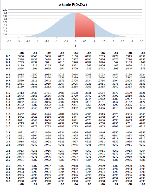
-table: The
-score table is used to calculate probabilities for the standard normal distribution.
From the table, we learn that:
Part two: For the second problem we have two values of
to standarize:
and
. Standardizing these values we obtain:
and
.
Notice that the first value is negative, which means that it is below the mean. Therefore:
Finding the Area Under the Normal Curve
To calculate the probability that a variable is within a range in the normal distribution, we have to find the area under the normal curve.
Learning Objectives
Interpret a
-score table to calculate the probability that a variable is within range in a normal distribution
Key Takeaways
Key Points
- To calculate the area under a normal curve, we use a
-score table. - In a
-score table, the left most column tells you how many standard deviations above the the mean to 1 decimal place, the top row gives the second decimal place, and the intersection of a row and column gives the probability. - For example, if we want to know the probability that a variable is no more than 0.51 standard deviations above the mean, we find select the 6th row down (corresponding to 0.5) and the 2nd column (corresponding to 0.01).
Key Terms
- z-score: The standardized value of observation
from a distribution that has mean
and standard deviation
.
To calculate the probability that a variable is within a range in the normal distribution, we have to find the area under the normal curve. In order to do this, we use a
-score table. (Same as in the process of standardization discussed in the previous section).

Areas Under the Normal Curve: This table gives the cumulative probability up to the standardized normal value
.
These tables can seem a bit daunting; however, the key is knowing how to read them.
- The left most column tells you how many standard deviations above the the mean to 1 decimal place.
- The top row gives the second decimal place.
- The intersection of a row and column gives the probability.
For example, if we want to know the probability that a variable is no more than 0.51 standard deviations above the mean, we find select the 6th row down (corresponding to 0.5) and the 2nd column (corresponding to 0.01). The intersection of the 6th row and 2nd column is 0.6950. This tells us that there is a 69.50% percent chance that a variable is less than 0.51 sigmas above the mean.
Notice that for 0.00 standard deviations, the probability is 0.5000. This shows us that there is equal probability of being above or below the mean.
Consider the following as a simple example: find
.
This problem essentially asks what is the probability that a variable is less than 1.5 standard deviations above the mean. On the table of values, find the row that corresponds to 1.5 and the column that corresponds to 0.00. This gives us a probability of 0.933.
The following is another simple example: find
.
This problem essentially asks what is the probability that a variable is MORE than 1.17 standard deviation above the mean. On the table of values, find the row that corresponds to 1.1 and the column that corresponds to 0.07. This gives us a probability of 0.8790. However, this is the probability that the value is less than 1.17 sigmas above the mean. Since all the probabilities must sum to 1:
As a final example: find
.
This example is a bit tougher. The problem can be rewritten in the form below.
The difficulty arrises from the fact that our table of values does not allow us to directly calculate
. However, we can use the symmetry of the distribution, as follows:
So, we can say that:
Licenses and Attributions
Source: https://www.coursehero.com/study-guides/boundless-statistics/the-normal-curve/